Evolving neural networks
Evolving neural networks
NeuroEvolution of Augmenting Topologies is a way to both create and train neural networks using genetic algorithms. It was introduced in 2002 by Kenneth O. Stanley and Risto Miikkulainen in the paper Evolving Neural Networks through Augmenting Topologies.
I implemented it with a few variations and heuristics of my own as my first real CS project.
Process overview
The main idea is very simple: a neural network is a graph, neurons are nodes and inter-neurons connections are weighted edges.
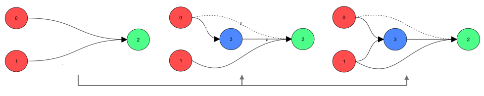
Start with a population of neural networks with random weights and the minimal structure: all the input nodes connected to all the output ones. Then, evolve in one of two way:
- A new node is added on an existing connection. The old one is deactivated.
- A new connection is created between two unconnected nodes.
After that, the weights are perturbed, similar individuals are crossed over to create new ones and finally, everyone is evaluated. Weak individuals are dismissed and the cycle starts over.
Summary
- Mutate the structure
- Perturb the weights
- Cross over
- Evaluate
- Select
Although the process is very straight forward, there’s one tricky part: crossing individuals over.
Subtleties
Crossing two paths in the travelling salesman problem is rather simple, crossing over two neural networks is inherently hard. For a crossover between neural networks to make sense, they must share a lot of common traits.
Innovation number
Each structural mutation (connection or neuron), also called gene, has a unique, increasing id: the “innovation number”. It must be the same even if a given mutation occurs in two neural networks with several generations (and thus mutations) in between.
Speciation
The distance between two individuals is then given by the following formula:
where:
- $E$ is the number of “Excess” genes, which innovation number excess the max one of the other individual.
- $D$ is the number of “Disjoint” genes, present in an individual and not in the other.
- $N$ is the total number of genes, including de-activated ones.
- $\bar{W}$ is the average weight difference.
- $c_1$, $c_2$, $c_3$ are arbitrary coefficients.
A threshold $d_s$ is used to infer species, i.e. groups of similar individuals, form the distance matrix. Cross-over is only allowed within species.
Cross-over rules
| Gene innovation number: | 1 | 2 | 3 | 4 | 5 | |
|---|---|---|---|---|---|---|
| Gene type: | common | disjoint | disjoint | common | excess | |
| Worse performing parent | x | x | x | |||
| Best performing parent | x | x | x | x | ||
| Offspring | x | x | x | x |
Keep original genes from the best parent, average the weights for common ones.
Stagnation and potential
If the fitness of a species does not increase enough over a generation, its stagnation is incremented. Whenever there’s a significant fitness leap the stagnation is reset.
The potential is the number used to attribute the number of offsprings to a species. It measures how dynamic the evolution of a species is.
Stagnant species have fewer offsprings, this strategy helps overcoming local fitness maximums.
Freezing the structure
At some stage of the training, the strucutre of the graph can be frozen and gradient descent used for a quicker convergence.