Transverse concepts

Probability things

• Null and alternative hypothesis : the null hypothesis $H_0$ describes the world (e.g. a parameter) when there’s nothing new under the sun.

• Type I error : rejection of a true null hypothesis, false positive.

• Type II error : non-rejection of a false null hypothesis, false negative.

• $p$-value: the probability $P(\textbf{x} | H_0)$ of obtaining the data under the null hypothesis. It measures the un-surprisingness of the evidence.

• independent and identically distributed (iid): set of mutually independent random variables with the same probability distribution

• Convergence in law / in distribution $X_n \overset{d}{\longrightarrow} X$:
  $\forall x, \quad F_n(x) \underset{n \to \infty}{\longrightarrow} F(x)$

• Convergence in probability $X_n \overset{p}{\longrightarrow} X$:
  $\forall \epsilon, \quad P(X_n - X > \epsilon) \underset{n \to \infty}{\longrightarrow} 0$

• Almost sure convergence $X_n \overset{a.s.}{\longrightarrow} X$:
  $P(X_n \underset{n \to \infty}{\longrightarrow} X) = 1$

• Weak law of large numbers:
  $\bar{X}_n \overset{p}{\longrightarrow} \mu$

• Strong law of large numbers:
  $\bar{X}_n \overset{a.s.}{\longrightarrow} \mu$

• Central limit theorem: Given $n$ iid random variable with an expected value $\mu$ and a variance $\sigma^2$
  $\sum X_i \overset{d}{\longrightarrow} \mathcal{N}(n\mu, \sqrt{n}\sigma^2)$

Information

The information of an event $I(E) = -log_2(P(E))$ captures the surprise of the event actually happening (base $2$ to express it in bits, $\ln$ to expresses it in nats))

The entropy is then defined as the expected value of information $H(X) = \mathbb{E}[I(X)]$. For instance the entropy of the probability distribution of an agent’s actions the uncertainty/chaos/entropy of his behavior, the uncertainty of a probability distribution.

Cross-entropy is a way to measure the “distance” (not symetric) between two distributions, which is useful when trying to approximate a distribution $P$ by another, $Q$. $H(p,q) = H(p) + D_{KL}(p ~||~ q)$.

The KL divergence measures the surprise of them being not close. The likelyhood ratio $\text{LR} = \frac{p(x)}{q(x)}$ is $> 1$ if the sample is most likely coming from $P$ and $<1$ otherwise. For $n$ sample we have $\text{LR} = \prod \frac{p(x_i)}{q(x_i)}$. The KL divergence is then expressed as $D_K~_L(p ~||~ q) = \sum p(x_i)\log(\frac{p(x_i)}{q(x_i)})$. $P$ being the “true” distribution, the KL divergence amounts of information lost when expressing it via $Q$.

Bayesian reasoning

In the context of classification, the Bayes theorem, $P(A | B) = \frac{P(B|A)P(A)}{P(B)}$, is often used as :

Bayes use case example

The brethalizer policemen use has a $5%$ false positive rate but never fails to detect a drunk driver. A driver is controled positive. What’s the probability of him being drunk ? $95%$ ?

Let’s assume that, a priori, about $0.1%$ of all the drivers are actually drunk (this is the Bayesian step, assuming prior knowledge).

The positive probability becomes

True positive + false positive (independance, being drunk doesn’t alter the brethalizer’s law).

We finally have

Doing the test several times will greatly increase the certainty of him being drunk. With 3 positive tests it is about $88%$.

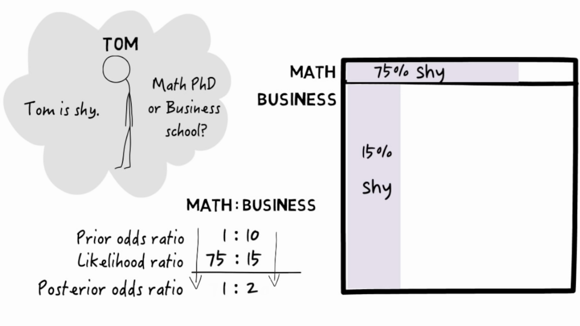
Odds

More practicaly with odds ($\text{Drunk} : \text{Sober}$):

• Prior odds of being drunk $1 : 999$
• Likelyhood of brethalizer positive $100 : 5$

$100 : 4995 = 20 : 999$ are actually drunk which is about a $\frac{20}{1019} = 2%$ probability.

Here is a visual example from Julia Galef. The ratios can be seen as areas of the total population.

Updating with additional data

If we do another test, we get $2000 : 4995 = 400 : 999$ odds of being drunk, which is also

With third test, the driver already has a $\approx 89%$ probability of being actually drunk.

Classification

When we know the classes the data can belong to.

One vs One and One versus Rest

To extend a binary decision algorithm to $n$ classes, either build $n$ binary classifier $\text{Class}_i$ vs $!\text{Class}_i$ or $n^2$ classifiers $\text{Class}_i$ vs $\text{Class}_j$ and “vote” to take the decision.
The algorithm must provide a way to evaluate the confidence in their predictions to resolve equalities in votes.

Decision trees

• Split the input space with conditions on the data e.g. x.1 >= 0 with a greedy approach. The decision is the majority class in the leaf.
• Split in order to have the purest child nodes (algos: CART, ID3, C4.5…).
• Impurity measures: $0$ when sets are pure and maximum when the class' proportions in the set are even.
  • Gini impurity $\text{I}_G(p) = \sum p_i(1-p_i)$ ranging from $0$ to $0.5$ is the probability of being wrong when randomly labeling an element according to the distributions of labels in the subset.
  • Maximize the Gini gain : substract the weighted (by the proportion of elements) sum of the childs' impurity to the impurity of the branch.
  • The entropy $H(X) \sum P(x_i)log(P(x_i))$ (in decision trees, $P(x_i) = p_i$ the proportion of individuals from the class $i$ in the node), measures the homogeneity of a sample. Entropy is equal to $1$ for even proportions and $0$ when pure.
  • Maximize the information gain : substract the entropy of the childs from that of the branch.
• Overfit then prune the tree by removing the nodes which doesn’t affect the test error, or stop at an information gain threshold / preset depth.
• Fully explainable, and that’s cool.
• Works well on small datasets

Random forests

• Have a set of decision trees make a prediction and average the result.
• To have different decision trees either train them on disjoint subsets of the dataset or constrain the features they can use.
• Needs more data than basic decision trees.

K-NN

• Find the $k$ closest known examples and predict the majority class.
• Supposes that the items being close known-features-wise implies that their unknown features are close too.
• Predictions are slow $O(|\text{train set}|)$.

Naive Bayes

• Naively supposes conditional independance between the features of the dataset given the class variable.

1. Pick a class to compute the probability of belonging to it.
2. Find the prior probability (often $\frac{\# \text{class}}{\# \text{subjects}}$)
3. Calculate the marginal likelihood, i.e. the probability of being equal or close to the new datapoint. It can be the proportion of the class in an arbitrary neighborhood of the new datapoint.

4. Compute the likelihood, _i.e._ the probability of being of the target class when being equal or close to the new datapoint. It can be the proportion of the class in the afore-defined neighborhood. 5. Compute the posterior probability with the Bayes formula: $\frac{\text{Likelihood} \times \text{Prior}}{\text{Marginal}}$. 6. Compute the posterior probabilities for the other classes. 7. Pick the class with the greatest probability.

• Good for non-linear data, datasets with outliers.
• The naive independance assuumption can create bias.

Logistic regression

1. Do a linear regression $y = b_0 + b^\top \textbf{x}$ with class A = $0$ and class B = $1$ and interpret the result as the likelihood of belonging to class B.
2. you want a probability from a sigmoid $p = \frac{1}{1 + e^{-y}}$
3. $\ln(\frac{p}{1-p}) = y = b_0 + b^\top \textbf{x}$, hence the probability is $p = \frac{1}{1 + e^{-b_0 + b^\top\textbf{x}}}$ and the odds are $\frac{p}{1-p} = e^{b_0 + b^\top \textbf{x}}$

• Can specify which variable is significant to make a prediction

Clustering

K-means

1. Select a number K of cluster
2. Use K random points as the first centroids
3. Assign each data point to the closest centroid
4. Compute the new centroids which are the center of mass of the current clusters
5. If a centroid moved go to 3.

• To evaluate the quality of a clustering, one can compute the Within Cluster Sum of Squares WCSS

• Pick the number of cluster K corresponding to an “elbow” in the $y = \text{WCSS}(K)$ curve.

Reinforcement learning

Notations

• $V(s)$ value of a state $s$.
• $Q(a)$ value of an action $a$.
• $N(a)$ number of times action $a$ has been selected.
• $_t$ at the (discrete) timestep $t$.
• $A$ action.
• $S$ action.

Bellman equations

The optimal value function of a state is the sum for all transitions of the immediate reward and the discounted optimal value of the state you land on weighted by their probability of the transition occuring when taking the best action.

where $0 < \gamma < 1$ is the discount factor which reduces the reward of future states.

The optimal value function of an action is the sum for all transitions of the immediate reward and the discounted value of the best action takeable from the target state weighted by their probability of the transition occuring when taking the action.

Upper Confidence Bound (UCB)

Gvien a multi-armed bandit (or a similar problem)

1. Make some trials to estimates the expected return for each arm and a confidence interval around them.
2. Use the arm which confidence interval has the highest upper bound.
3. Update (narrow) the confidence interval after each trial.

• As the used interval will narrow, its upper bound may go below another. Ultimately the algorithm will end up using only the optimal arm.

where $c$ controls the degree of exploration, and can be set according to prior knowledge of the distribution e.g. 1.96 for a 95% confidence interval under a gaussian prior.

Thompson sampling

• Essentially, replace the confidence intervals of the UCB by normal distributions centered on the estimated expected returns.

1. Sample an expected return from each distribution, these are our beliefs about the actual expected returns.
2. Use the armed which is believed to have the highest expected return.
3. Update (narrow) the distribution.

Policy evaluation